Interpretability: Inferring importances for GO and genes#
NetworkVI is a Variational Autoencoder for the paired and mosaic integration of multimodal single-cell data. Each single-cell modality is learned in individual encoders; the latent spaces are then aligned for a joint representation. In this notebook we demonstrate how to use the inherent interpretability of NetworkVI to infer importances for GO terms and genes. We use a publically available CITE-seq dataset created by [LBC+21].
If you use NetworkVI, please consider citing:
Arnoldt, L., Upmeier zu Belzen, J., Herrmann, L., Nguyen, K., Theis, F.J., Wild, B. , Eils, R., “Biologically Guided Variational Inference for Interpretable Multimodal Single-Cell Integration and Mechanistic Discovery”, bioRxiv, June 2025.
import os
import sys

IN_COLAB = "google.colab" in sys.modules

if IN_COLAB:
    !pip install networkvi
import warnings
from sklearn.exceptions import ConvergenceWarning
warnings.filterwarnings("ignore")
warnings.filterwarnings("ignore", category=ConvergenceWarning)
warnings.filterwarnings("ignore", message="Liblinear failed to converge")
import numpy as np
import requests
import sys
sys.path.append("../../src")
import networkvi
from networkvi.model import NETWORKVI
import scanpy as sc
import anndata as ad
import matplotlib.pyplot as plt
from sklearn.ensemble import RandomForestClassifier
import sklearn
from sklearn.preprocessing import normalize
import seaborn as sns
import pandas as pd
from goatools.obo_parser import GODag
import shutil
%matplotlib inline
os.makedirs("../../resources/", exist_ok=True)
if not os.path.isfile(os.path.join("../../resources/", "go-basic.obo")):
    r = requests.get("http://purl.obolibrary.org/obo/go/go-basic.obo", allow_redirects=True)
    open(os.path.join("../../resources/", "go-basic.obo"), 'wb').write(r.content)
gene_csv_path = "../../gene_interactions.csv"
gene_csv_url = "https://zenodo.org/records/19376389/files/ENCFF173VDJ_K562_GRCh38_contact_domains_juicertools.csv?download=1"

if not os.path.isfile(gene_csv_path):
    print(f"Downloading {gene_csv_path} from Zenodo...")
    r = requests.get(gene_csv_url)
    r.raise_for_status()
    with open(gene_csv_path, "wb") as f:
        f.write(r.content)
    print("Download complete.")
Data loading#
We provide a subsetted and preprocessed version of the CITE-seq and Multiome dataset for this tutorial. We filtered low qualty cells, lowly expressed features and performed subsampling to 5000 cells and feature subselection to 4000 highly variable genes and 20000 highly variable ATAC peaks. NetworkVI accepts raw counts data for all modalities. For details on the preprocessing please refer to the manuscript and the code in the NetworkVI reproducibility repository. In the repository we also provide scripts for downloading and processing the datasets used in the manuscript. The original CITE-seq dataset contains 90261 bone marrow mononuclear cells inferred at 4 different sites with 13953 genes and 143 proteins.
rna_cite_path = "neurips2021_cite_bmmc_luecken2021.h5ad"

try:
    rna_cite = sc.read_h5ad(rna_cite_path)
except OSError:
    import gdown

    gdown.download("https://drive.google.com/uc?export=download&id=1A9o8wZgWS6udFMXJ-ybXre1dCcCdsKt5")
    rna_cite = sc.read_h5ad(rna_cite_path)

rna_cite
AnnData object with n_obs × n_vars = 5000 × 4000
    obs: 'cell_type', 'Site', 'DonorID', 'DonorSmoker', 'DonorBMI', 'DonorAge'
    var: 'gene_stable_id', 'modality'
    uns: 'protein_expression'
    obsm: 'protein_expression'
Data setup#
To perform query-to-reference mapping, we select the cells inferred at one of the four different sites as the query dataset. We train NetworkVI on the rest of the dataset.
adata = rna_cite
query = adata[adata.obs["Site"] == "site1"].copy()
adata = adata[adata.obs["Site"] != "site1"].copy()
We register the fields and setup the anndata with a convenience function as shown below. NetworkVI requires as MultiVI to register the modality as the batch_key. Further batch information can be registered as categorical_covariate_keys.
NETWORKVI.setup_anndata(
    adata,
    batch_key="Site",
    protein_expression_obsm_key="protein_expression",
)
Model setup and training#
We demonstrate the setup and training of NetworkVI, which makes use of the Gene Ontology, as the encoder structure. Below we define a convenience function to get the latent representation and to visualize the latent space. NetworkVI requires as MultiVI the definition of the number of features per modality (n_genes, n_proteins, n_regions).
def get_plot_latent_representation(vae, adata):
    latent_representation = vae.get_latent_representation(modality="joint")
    adata.obsm["X_NetworkVI"] = latent_representation
    sc.pp.neighbors(adata, use_rep="X_NetworkVI")
    sc.tl.umap(adata, n_components=2)
    return adata
NetworkVI#
We select NetworkVI by setting layers_encoder_type to “go”. The mapping of the features to the gene layer and the Gene Ontology requires ENSEMBL-IDs, which we provide in ensembl_ids_genes and ensembl_ids_proteins. We also provide the Gene Ontology and a gene-to-GO mapping file in obo_file and map_ensembl_go. Please don’t use the provided mapping file in production since it’s an artifically subsampled version of a real mapping file. Please refer to the scripts provided here or here to download full mapping files.
vae = NETWORKVI(
    adata,
    n_genes=len(adata.var[adata.var["modality"] == "Gene Expression"]),
    n_proteins=adata.obsm["protein_expression"].shape[1],
    ensembl_ids_genes=np.array(adata.var[adata.var["modality"] == "Gene Expression"]["gene_stable_id"]),
    ensembl_ids_proteins=np.array(adata.uns["protein_expression"]["var"]["gene_stable_id"]),
    gene_layer_interaction_source="../../gene_interactions.csv",
    expression_gene_layer_type="interaction",
    protein_gene_layer_type="interaction",
    obo_file="../../resources/go-basic.obo",
    map_ensembl_go=["../../resources/ensembl2go.gaf"],
    layers_encoder_type="go",
    encode_covariates=True,
    deeply_inject_covariates=True,
    fully_paired=True,
    standard_gene_size=5,
    standard_go_size=2,
)

vae.train(max_epochs=10, adversarial_mixing=False, save_best=False)
Generated block structure with len 4000 (0.00025 blocks).
Generated block structure with len 7342 (0.000458875 blocks).
../../resources/go-basic.obo: fmt(1.2) rel(2025-03-16) 43,544 Terms; optional_attrs(relationship)
../../resources/go-basic.obo: fmt(1.2) rel(2025-03-16) 43,544 Terms; optional_attrs(relationship)
_biological_process_go-basic_ensembl2go.v2_processed.pkl
Using attention in GO model at level -1.
Generated block structure with len 4565 (0.07608333333333334 blocks).
Generated block structure with len 4565 (0.07608333333333334 blocks).
Using attention in GO model at level 1.
Generated block structure with len 18 (0.13333333333333333 blocks).
Generated block structure with len 18 (0.13333333333333333 blocks).
Generated block structure with len 297 (0.00825 blocks).
Generated block structure with len 297 (0.00825 blocks).
Using attention in GO model at level 0.
Generated block structure with len 1 (0.06666666666666667 blocks).
Generated block structure with len 1 (0.06666666666666667 blocks).
Generated block structure with len 8 (0.8888888888888888 blocks).
Generated block structure with len 8 (0.8888888888888888 blocks).
Generated block structure with len 134 (0.0078125 blocks).
Generated block structure with len 154 (0.0093994140625 blocks).
../../resources/go-basic.obo: fmt(1.2) rel(2025-03-16) 43,544 Terms; optional_attrs(relationship)
../../resources/go-basic.obo: fmt(1.2) rel(2025-03-16) 43,544 Terms; optional_attrs(relationship)
Using attention in GO model at level -1.
Generated block structure with len 182 (0.109375 blocks).
Generated block structure with len 182 (0.109375 blocks).
Using attention in GO model at level 1.
Generated block structure with len 16 (0.15384615384615385 blocks).
Generated block structure with len 16 (0.15384615384615385 blocks).
Generated block structure with len 27 (0.0263671875 blocks).
Generated block structure with len 27 (0.0263671875 blocks).
Using attention in GO model at level 0.
Generated block structure with len 1 (0.07692307692307693 blocks).
Generated block structure with len 1 (0.07692307692307693 blocks).
Generated block structure with len 7 (0.875 blocks).
Generated block structure with len 7 (0.875 blocks).
Training:   0%|                                                                                                         | 0/10 [00:00<?, ?it/s]
Epoch 1/10:   0%|                                                                                                       | 0/10 [00:00<?, ?it/s]
Epoch 1/10:  10%|█████████▌                                                                                     | 1/10 [00:05<00:51,  5.72s/it]
Epoch 1/10:  10%|███▌                               | 1/10 [00:05<00:51,  5.72s/it, v_num=1, train_loss_step=1.94e+4, train_loss_epoch=1.15e+4]
Epoch 2/10:  10%|███▌                               | 1/10 [00:05<00:51,  5.72s/it, v_num=1, train_loss_step=1.94e+4, train_loss_epoch=1.15e+4]
Epoch 2/10:  20%|███████                            | 2/10 [00:11<00:44,  5.59s/it, v_num=1, train_loss_step=1.94e+4, train_loss_epoch=1.15e+4]
Epoch 2/10:  20%|███████                            | 2/10 [00:11<00:44,  5.59s/it, v_num=1, train_loss_step=8.75e+3, train_loss_epoch=9.79e+3]
Epoch 3/10:  20%|███████                            | 2/10 [00:11<00:44,  5.59s/it, v_num=1, train_loss_step=8.75e+3, train_loss_epoch=9.79e+3]
Epoch 3/10:  30%|██████████▌                        | 3/10 [00:16<00:38,  5.54s/it, v_num=1, train_loss_step=8.75e+3, train_loss_epoch=9.79e+3]
Epoch 3/10:  30%|██████████▌                        | 3/10 [00:16<00:38,  5.54s/it, v_num=1, train_loss_step=1.03e+4, train_loss_epoch=8.63e+3]
Epoch 4/10:  30%|██████████▌                        | 3/10 [00:16<00:38,  5.54s/it, v_num=1, train_loss_step=1.03e+4, train_loss_epoch=8.63e+3]
Epoch 4/10:  40%|██████████████                     | 4/10 [00:22<00:33,  5.51s/it, v_num=1, train_loss_step=1.03e+4, train_loss_epoch=8.63e+3]
Epoch 4/10:  40%|██████████████▍                     | 4/10 [00:22<00:33,  5.51s/it, v_num=1, train_loss_step=9.7e+3, train_loss_epoch=7.74e+3]
Epoch 5/10:  40%|██████████████▍                     | 4/10 [00:22<00:33,  5.51s/it, v_num=1, train_loss_step=9.7e+3, train_loss_epoch=7.74e+3]
Epoch 5/10:  50%|██████████████████                  | 5/10 [00:27<00:27,  5.49s/it, v_num=1, train_loss_step=9.7e+3, train_loss_epoch=7.74e+3]
Epoch 5/10:  50%|███████████████████                   | 5/10 [00:27<00:27,  5.49s/it, v_num=1, train_loss_step=4.84e+3, train_loss_epoch=7e+3]
Epoch 6/10:  50%|███████████████████                   | 5/10 [00:27<00:27,  5.49s/it, v_num=1, train_loss_step=4.84e+3, train_loss_epoch=7e+3]
Epoch 6/10:  60%|██████████████████████▊               | 6/10 [00:33<00:22,  5.55s/it, v_num=1, train_loss_step=4.84e+3, train_loss_epoch=7e+3]
Epoch 6/10:  60%|█████████████████████              | 6/10 [00:33<00:22,  5.55s/it, v_num=1, train_loss_step=6.62e+3, train_loss_epoch=6.41e+3]
Epoch 7/10:  60%|█████████████████████              | 6/10 [00:33<00:22,  5.55s/it, v_num=1, train_loss_step=6.62e+3, train_loss_epoch=6.41e+3]
Epoch 7/10:  70%|████████████████████████▌          | 7/10 [00:38<00:16,  5.56s/it, v_num=1, train_loss_step=6.62e+3, train_loss_epoch=6.41e+3]
Epoch 7/10:  70%|█████████████████████████▏          | 7/10 [00:38<00:16,  5.56s/it, v_num=1, train_loss_step=6.8e+3, train_loss_epoch=5.93e+3]
Epoch 8/10:  70%|█████████████████████████▏          | 7/10 [00:38<00:16,  5.56s/it, v_num=1, train_loss_step=6.8e+3, train_loss_epoch=5.93e+3]
Epoch 8/10:  80%|████████████████████████████▊       | 8/10 [00:44<00:11,  5.53s/it, v_num=1, train_loss_step=6.8e+3, train_loss_epoch=5.93e+3]
Epoch 8/10:  80%|████████████████████████████▊       | 8/10 [00:44<00:11,  5.53s/it, v_num=1, train_loss_step=4.1e+3, train_loss_epoch=5.52e+3]
Epoch 9/10:  80%|████████████████████████████▊       | 8/10 [00:44<00:11,  5.53s/it, v_num=1, train_loss_step=4.1e+3, train_loss_epoch=5.52e+3]
Epoch 9/10:  90%|████████████████████████████████▍   | 9/10 [00:49<00:05,  5.53s/it, v_num=1, train_loss_step=4.1e+3, train_loss_epoch=5.52e+3]
Epoch 9/10:  90%|███████████████████████████████▌   | 9/10 [00:49<00:05,  5.53s/it, v_num=1, train_loss_step=3.13e+3, train_loss_epoch=5.16e+3]
Epoch 10/10:  90%|██████████████████████████████▌   | 9/10 [00:49<00:05,  5.53s/it, v_num=1, train_loss_step=3.13e+3, train_loss_epoch=5.16e+3]
Epoch 10/10: 100%|█████████████████████████████████| 10/10 [00:55<00:00,  5.51s/it, v_num=1, train_loss_step=3.13e+3, train_loss_epoch=5.16e+3]
Epoch 10/10: 100%|█████████████████████████████████| 10/10 [00:55<00:00,  5.51s/it, v_num=1, train_loss_step=3.19e+3, train_loss_epoch=4.86e+3]
Epoch 10/10: 100%|█████████████████████████████████| 10/10 [00:55<00:00,  5.53s/it, v_num=1, train_loss_step=3.19e+3, train_loss_epoch=4.86e+3]
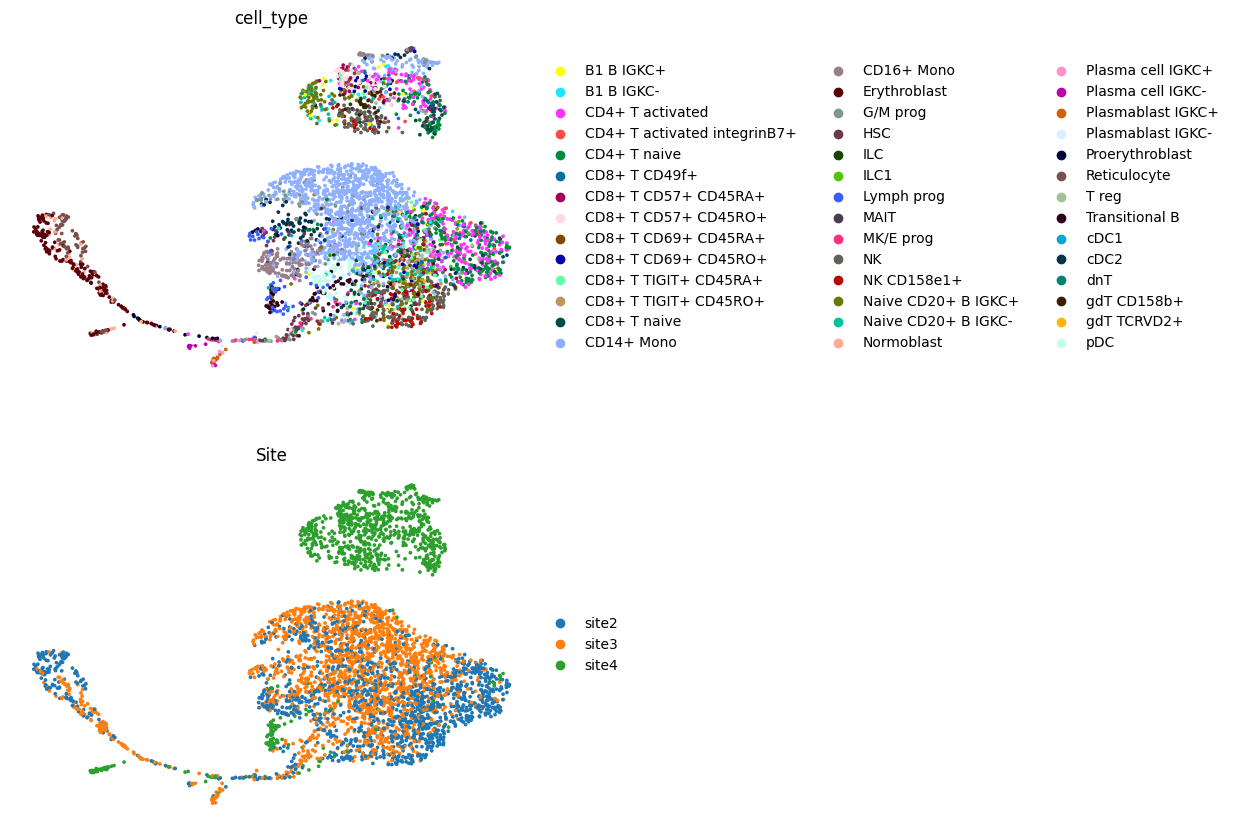
We can visualize the generated latent space:
adata = get_plot_latent_representation(vae, adata)
sc.pl.umap(adata, color=["cell_type", "Site"], frameon=False, ncols=1)
Interpretability#
By fitting a Logistic Regression on the activations of the nodes representing a GO term (calc_go_terms), a gene (calc_genes) or a gene_group (calc_gene_groups) we may infer the importance of this node for the performance of the neural network as described previously by [MYF+18]. Here, we demonstrate how to utilize the get_go_gene_importances and get_perturbation_go_gene_importances functions to infer the importances for the original dataset and for perturbed datasets in a sensitivity analysis. The importance is calculated in standard mode for each label against the rest. Using labels_selection, labels_selection_groups, restrict_by_column_key_activations_mask, restrict_by_column_values_activations_mask and comparison this behaviour may be modified. Please refer to the API documentation.
obodag = GODag(os.path.join("../../resources/", "go-basic.obo"))
../../resources/go-basic.obo: fmt(1.2) rel(2025-03-16) 43,544 Terms
_ = vae.get_go_gene_importances(labels_column="cell_type",
                                results_dir=f"tutorial/calc_go_terms",
                                shuffle_set_split=False,
                                batch_size=512,
                                calc_go_terms=True,
                                calc_genes=False,
                                calc_gene_groups=False,
                                save_fit=False)
Important Note on Logistic Regression Convergence
In this tutorial, we use a deliberately small, subsampled dataset (5,000 cells with 4,000 genes) to enable quick demonstration of NetworkVI’s interpretability features. This small dataset size has important implications for the downstream logistic regression analysis: When fitting logistic regression models to infer GO term and gene importances, you may encounter convergence warnings from scikit-learn’s Liblinear solver. These warnings are expected and not problematic for this tutorial because:
Limited separation between classes: With only a small subset of cells per cell type and a limited number of genes mapped to each GO term (often just 2-12 genes), there may be insufficient signal for the logistic regression to find clear decision boundaries between cell types for many GO terms.
Small sample sizes per GO term: Many GO terms in this subsampled dataset are represented by very few genes, making it mathematically difficult for the classifier to converge to an optimal solution.
Tutorial purposes: The goal here is to demonstrate the methodology for interpretability analysis, not to draw biological conclusions from this small dataset.
For production use: When applying NetworkVI to full-scale datasets with tens of thousands of cells and comprehensive gene coverage, convergence issues are much less common as there is substantially more signal for the logistic regression models to learn from. The warnings have been suppressed in this notebook to improve readability, but the underlying convergence behavior remains the same.
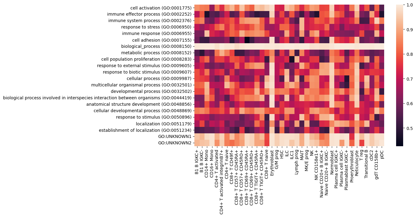
The function get_go_gene_importances saves the activations, GO importances and further information in a pandas pickle file. We then load these files and visualize the GO importance for a selection of GO terms for all available cell types.
go_importances = []
cell_types = []
for cell_type in sorted(np.unique(adata.obs["cell_type"])):
    cell_type_mod = cell_type.replace(" ", "_").replace("/", "_")
    try:
        go_importances.append(np.array(pd.read_pickle(f"./tutorial/calc_go_terms/protein_cell_type_vs_rest_{cell_type_mod}_res_unp_act_mask_False_flip_False_go_terms_evaluated_graph_csv.pkl")["predictors_label_valid_roc"]).astype("float"))
        cell_types.append(cell_type)
    except FileNotFoundError:
        continue
Please note that the loaded table does not only include the ROCs in the column predictors_label_valid_roc, but also the 95% CI for the ROCs in the columns predictors_label_valid_roc_ci_lower and predictors_label_valid_roc_ci_upper. For simplicitly, we do not demonstrate the 95% CI here, which on a dataset of this size, would indicate clear limitations of GO interpretability.
go_terms = list(pd.read_pickle(f"./tutorial/calc_go_terms/protein_cell_type_vs_rest_{cell_type_mod}_res_unp_act_mask_False_flip_False_go_terms_evaluated_graph_csv.pkl").index)
go_terms = [f"{obodag[go_term].name} ({go_term})" if go_term in obodag.keys() else go_term for go_term in go_terms]
plt.figure(figsize=(10, 6))

sns.heatmap(np.array(go_importances).T, xticklabels=cell_types, yticklabels=go_terms)
plt.show()
shutil.rmtree("tutorial/calc_go_terms")
We also show how to perform a sensitivity analysis by perturbing features. Here we perturb CD86 (ENSG00000114013) by setting all values to zero. The function get_perturbation_go_gene_importances internally calls get_go_gene_importances, but additionally we need to provide the modality of the features in modality_key and the ENSEMBL-IDs in gene_stable_id_key.
perturbation_gene_stable_ids = ["ENSG00000114013"]

go_importances_perturbation = vae.get_perturbation_go_gene_importances(labels_column="cell_type",
                                               modality_key="modality",
                                               gene_stable_id_key="gene_stable_id",
                                               perturbation_gene_stable_ids=perturbation_gene_stable_ids,
                                               batch_size=512,
                                               shuffle_set_split=False,
                                               calc_go_terms=True,
                                               calc_genes=False,
                                               calc_gene_groups=False,)
We can visualize the change of the importance in comparison to the not-perturbed dataset accordingly:
go_importances_pert = []

for cell_type in cell_types:
    cell_type_mod = cell_type.replace(" ", "_").replace("/", "_")
    go_importances_pert.append(go_importances_perturbation["ENSG00000114013"]['protein']["protein"][cell_type_mod]["roc"].astype("float"))
plt.figure(figsize=(10, 6))

sns.heatmap((np.array(go_importances) - np.array(go_importances_pert)).T, xticklabels=cell_types, yticklabels=go_terms)
plt.show()
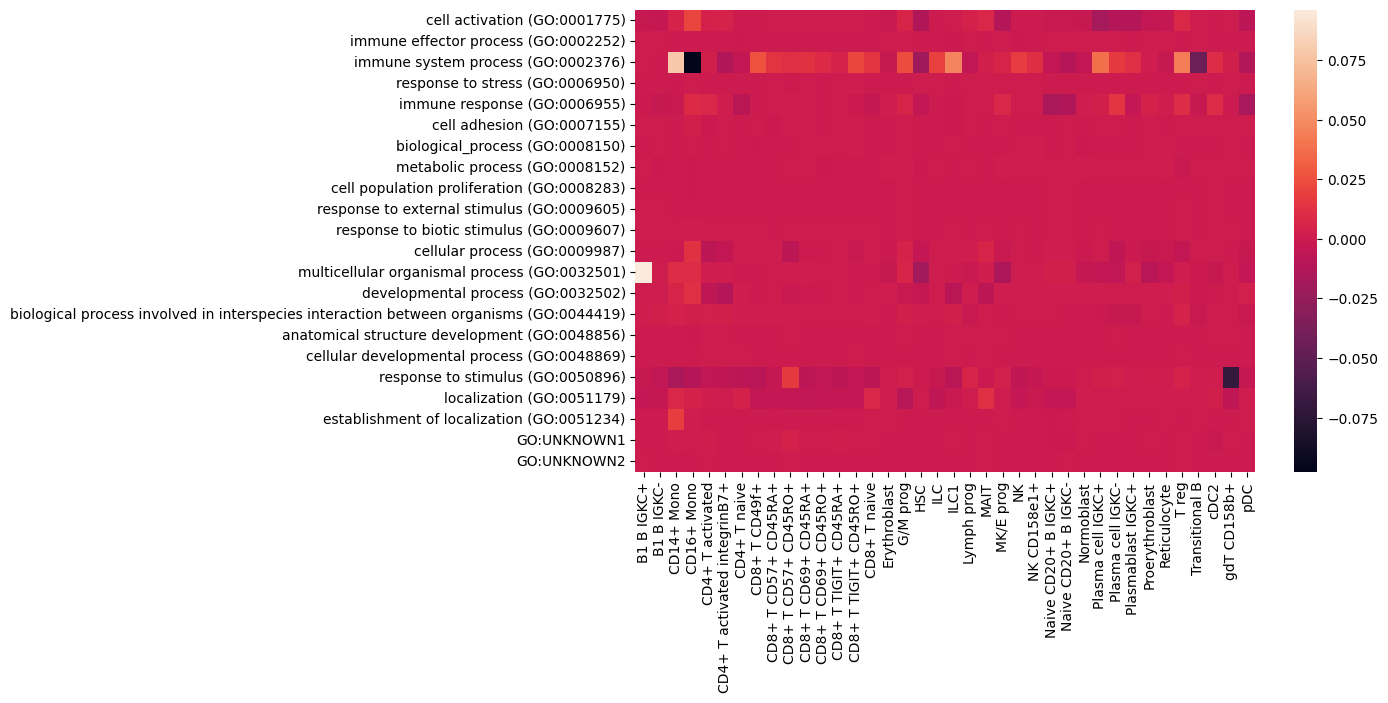
Please note, that again the dict contains not only the ROC values, but also the 95% CI lower and upper ROC values:
go_importances_perturbation["ENSG00000114013"]['protein']["protein"][cell_type_mod].keys()
dict_keys(['roc', 'roc_ci_median', 'roc_ci_lower', 'roc_ci_upper'])